Rolling Thunder Bicycles Company

1. Identifying Root Cause for Quality Issues and Estimate Overall Cost

1.1 Retrieve the Data

1.1.1 Tag the defected bicycles

We can make fully use of the Customer ID of whose bicycles are defected to find out which parts of the bicycle are in the wrong way.

Add a column named isDefect to tag whether the bicycle is defected.

SELECT iif(B.CustomerID in (26160, 40505, 29577, 40579, 18043, 41008, 2281, 40791, 40686, 40539, 875, 288, 40523, 29422, 40796), 1, Null) AS isDefect, * FROM Bicycle AS B;

1.2 Analyze the Data

1.2.1 Possible root cause: Category and Manufacturer

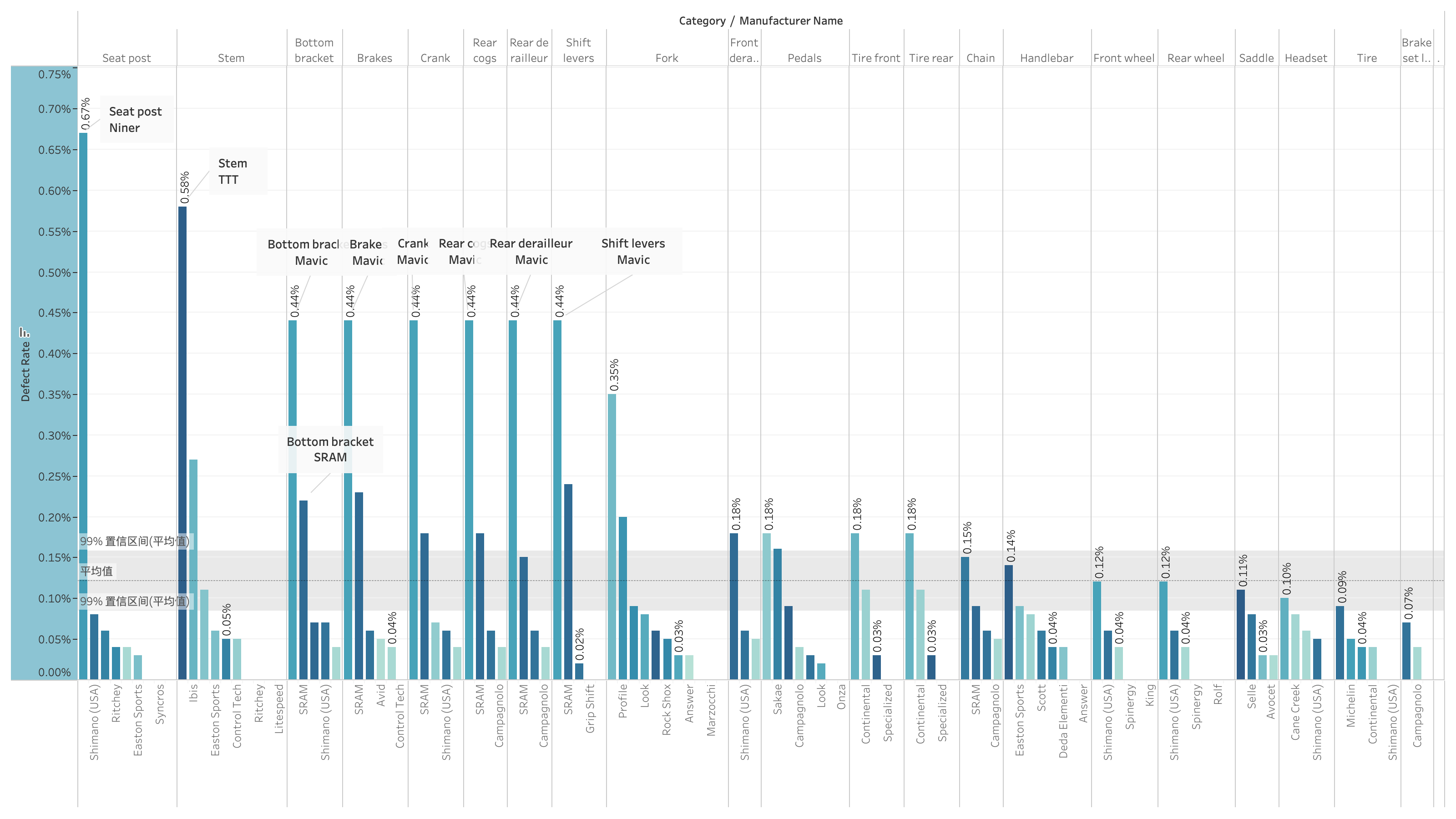
Calculate the defect rate of each category of component produced by different manufacturer.

Based on 95% Confidence Interval, the defect rate to Shimano’ seat post, TTT’s stem, Mavic’s Bottom bracket, brakes, crank, rear cogs, rear de railleur and shift levers, Fork, and ... (defect rate greater than 0.16%) are irregular value.

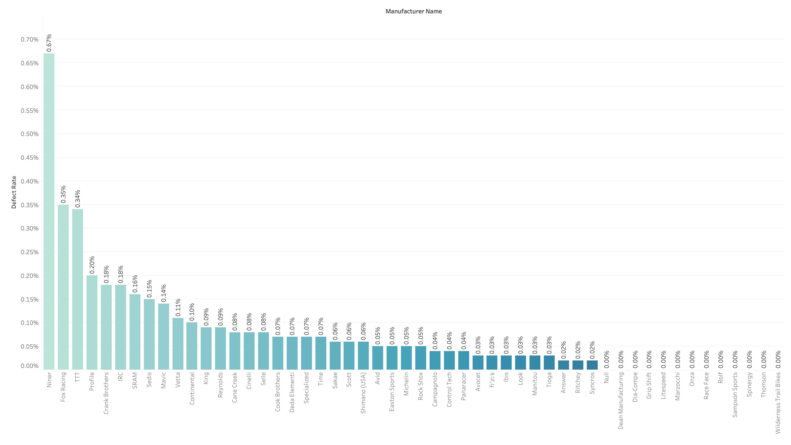
And manufacturer Niner, Fox Racing, TTT and Profile produced high defect rate components(defect rate greater than 0.30%), which worth great attention.

SELECT Category, B.ManufacturerID AS ManufacturerID, B.ManufacturerName AS ManufacturerName, count(*) AS TotalProduction, count(B.isDefect) AS TotalDefected, FormatPercent(count(B.isDefect) / count(*)) AS DefectRate
FROM (SELECT B.SerialNumber as SerialNumber, BP.ComponentID as ComponentID, C.Category as Category, M.ManufacturerID as ManufacturerID, M.ManufacturerName as ManufacturerName, B.isDefect as isDefect
FROM S1 AS B, BikeParts AS BP, Manufacturer AS M, Component AS C
WHERE (B.SerialNumber = BP.SerialNumber) and (M.ManufacturerID = C.ManufacturerID) and (BP.ComponentID = C.ComponentID))  AS B
GROUP BY B.Category, B.ManufacturerID, B.ManufacturerName
ORDER BY round(count(B.isDefect) / count(*) * 100, 2) DESC;

SELECT B.ManufacturerID AS ManufacturerID, B.ManufacturerName AS ManufacturerName, count(*) AS TotalProduction, count(B.isDefect) AS TotalDefected, FormatPercent(count(B.isDefect) / count(*)) AS DefectRate
FROM (SELECT B.SerialNumber as SerialNumber, BP.ComponentID as ComponentID, C.Category as Category, M.ManufacturerID as ManufacturerID, M.ManufacturerName as ManufacturerName, B.isDefect as isDefect
FROM S1 AS B, BikeParts AS BP, Manufacturer AS M, Component AS C
WHERE (B.SerialNumber = BP.SerialNumber) and (M.ManufacturerID = C.ManufacturerID) and (BP.ComponentID = C.ComponentID))  AS B
GROUP BY B.ManufacturerID, B.ManufacturerName
ORDER BY round(count(B.isDefect) / count(*) * 100, 2) DESC;

1.2.2 Possible root cause: Group

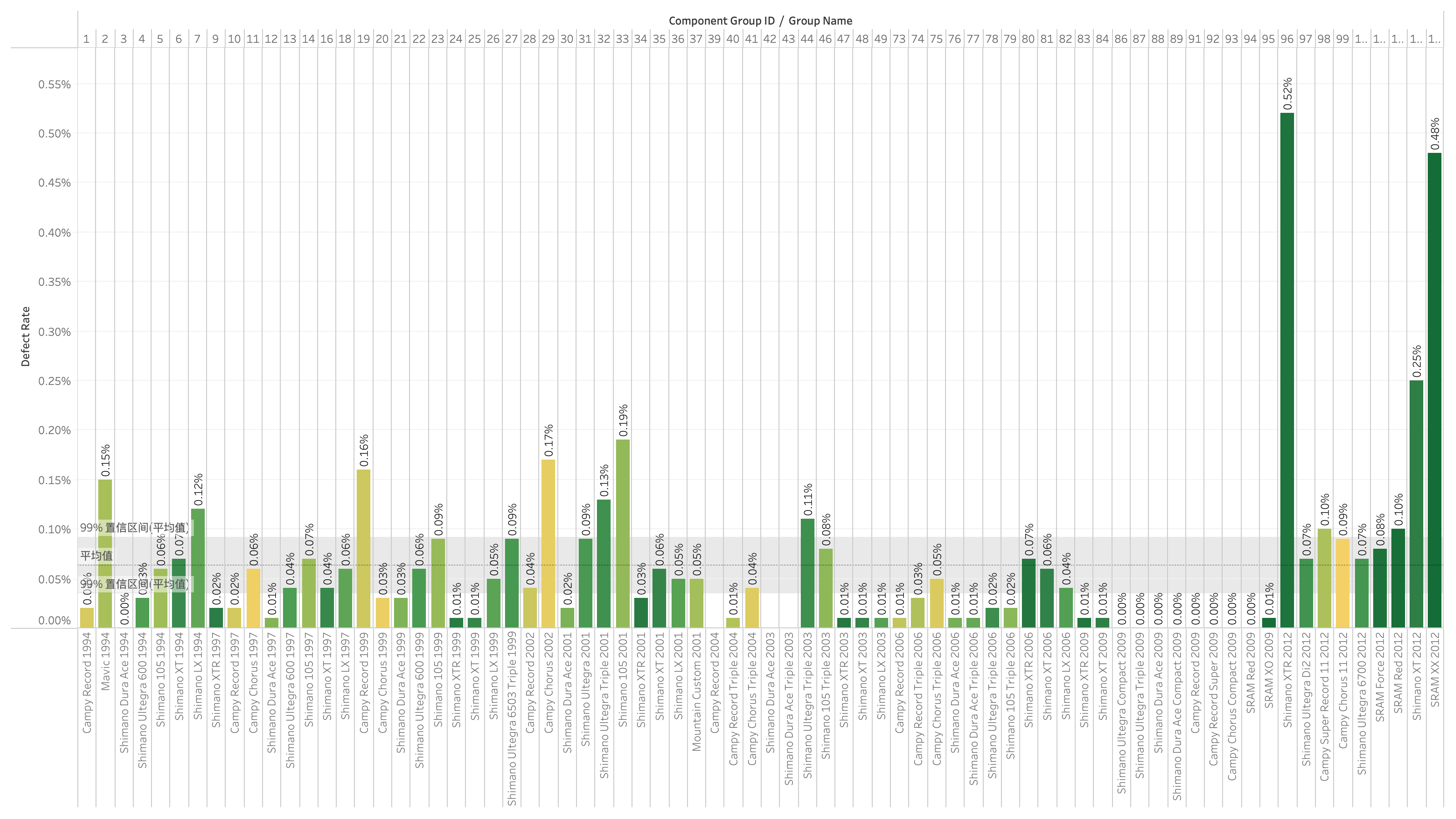
Each components are produced in different groups. Calculate the defect rate of each group.

Based on 95% Confidence Interval, some defect rate are abnormal (greater than 0.10%). They are from Group 2, 7, 19, 29, 33, 34, 44, 96, 98, 102, 103 and 104 (Group ID).

1.2.3 Possible root cause: ModelType and Material

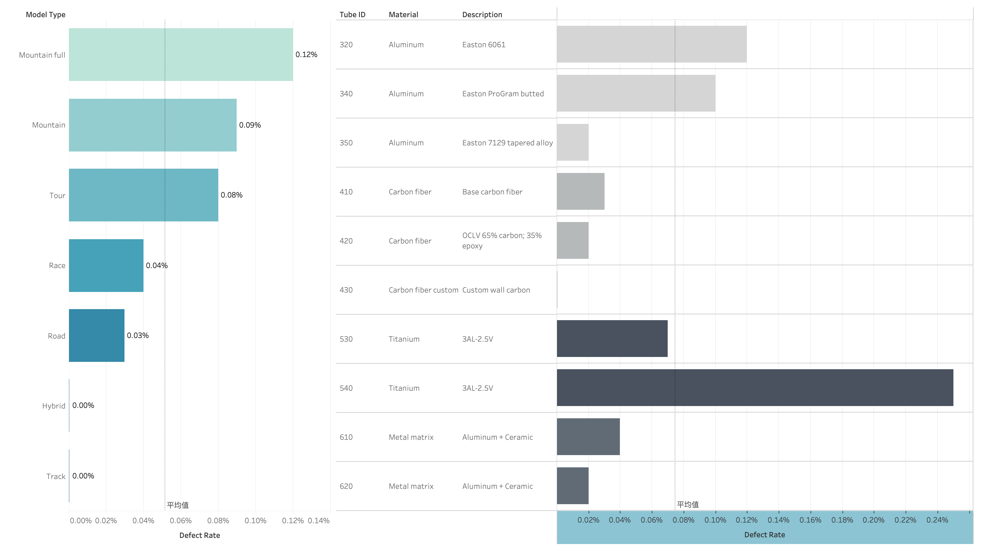
Calculate the defect rate of seven types of bicycle model type and the defect rate of each material used to build the bicycle.

The ModelType of Mountain full has the highest defect rate. There is no defected bicycles in the ModelType of Hybrid and Track.

Among different materials, the Titanium material with Tube ID 540 performs badly. And the Aluminum material with Tube ID 320 has a high defect rate either. These two types of materials are suspicious.

SELECT S.ModelType, count(*) AS Total, count(S.isDefect) AS Defects, FormatPercent(Defects / Total) AS DefectRate
FROM S1 AS S
GROUP BY S.ModelType
ORDER BY count(S.isDefect) / count(*) DESC;

1.2.4 Suspicious bicycles

Some manufacturer, category of Components, component group, model type and material of the bicycle’s frame have high defect rate. Based on 95% confident interval of each option, we can set a standard (table below) to select bicycles in all of the high defect rate options. Those bicycles are suspected to have internal quality issues.

	Manufacturer	Manufacturer Category	Group	ModelType	Material
Defect Rate	>0.30%	>0.16%	>0.10%	>0.08%	>0.08%

SELECT B.OrderDate, B.SerialNumber, B.SalePrice, B.ShipPrice, ComponentList, B.FramePrice, C.EstimatedCost, C.ListPrice, C.Category, C.ManufacturerID, GC.GroupID
FROM Bicycle AS B, BikeParts AS BPs, Component AS C, GroupComponents AS GC, BicycleTubeUsage AS BT
WHERE B.SerialNumber = BPs.SerialNumber and BPs.ComponentID = C.ComponentID and GC.ComponentID = C.ComponentID and B.SerialNumber = BT.SerialNumber and
(
(C.Category = 'Seat post' and C.ManufacturerID = 68) or
(C.Category = 'Stem' and C.ManufacturerID in (46, 48)) or
(C.Category = 'Bottom bracket' and C.ManufacturerID in (8, 53)) or
(C.Category = 'Brakes' and C.ManufacturerID in (8, 53)) or
(C.Category = 'Crank' and C.ManufacturerID in (8, 53)) or
(C.Category = 'Rear derailleur' and C.ManufacturerID in (8)) or
(C.Category = 'Shift levers' and C.ManufacturerID in (8, 53)) or
(C.Category = 'Fork' and C.ManufacturerID in (58, 14)) or
(C.Category = 'Rear derailleur' and C.ManufacturerID in (53)) or
(C.Category = 'Pedals' and C.ManufacturerID in (59, 11)) or
(C.Category = 'Rear derailleur' and C.ManufacturerID in (53)) or
(C.Category = 'Tire front' and C.ManufacturerID in (65)) or
(C.Category = 'Tire rear' and C.ManufacturerID in (65))
) and
GC.GroupID in (2, 7, 19, 29, 32, 33, 44, 96, 98, 102, 103, 104) and
BT.TubeID in (320, 340, 540) and
B.Modeltype in ('Mountain full', 'Mountain', 'Tour') and
C.ManufacturerID in (68, 58, 46)
ORDER BY B.SerialNumber;

1.2.5 Recalled plan

It is sure that these bicycles should be recalled. After recalling them, there are two plans to deal with them: replace the suspicious components or sent customer’s money back.

If choose the former plan, the company need to pay for the ship price and the component price. The minimum cost of the repaired component is the estimated price of it, the maximum cost of the repaired component is its listed price.

If choose the latter plan, the company need to pay for the ship price and the sale price customer paid.

Using SQL, we can calculate the cost for each plan.

Recall	Minimum	Maximum
$4,806,180.00	$844,164.20	$1,332,050.00

select SerialNumber, (SalePrice + ShipPrice) as Resent, (sum(EstimatedCost) + ShipPrice) as Min, (sum(ListPrice) + ShipPrice) as Max
from S11
group by SerialNumber, SalePrice, ShipPrice, ComponentList, FramePrice;

select sum(Resent) as Recall, sum(Min) as Minimum, sum(Max) as Maximum
from S11_Recall;

1.3 Conclusion

1.3.1 Possible root cause

The Manufacturer, Category and Manufacturer of component, manufacturing group, bicycle’s modeltype and bicycle’s material are possible root cause. If any of them of one bicycle meet the condion in the table in 1.2.4, this bicycle are regarded as having an internal quality issue.

1.3.2 Recall

If the company choose to recall the possible bad bicycles and sent customer’s money back, the cost is approximately $4,806,180.

If the company choose to recall the possible bad bicycles and replace their components, the cost is estimated between $844,164 and $1,332,050.

2. Forecasting for Capacity Expansion

2.1 Retrieve the Data

2.1.1 Data processing

SELECT B.OrderDate, Year([B.OrderDate]) AS [Year], Month([B.OrderDate]) AS [Month], Day([B.OrderDate]) AS [Day], B.ModelType AS ModelType, B.FrameSize AS FrameSize, B.LetterStyleID AS LetterStyle, P.ColorName AS Color, C.City AS City, count(*) AS Amount, sum(B.SalePrice) AS TotalSell, (sum(B.SalePrice) - sum(B.SalesTax) - sum(B.ShipPrice) - sum(B.FramePrice) - sum(B.ComponentList)) AS Profit
FROM Bicycle AS B, Paint AS P, RetailStore AS R, City AS C
WHERE (B.PaintID = P.PaintID) and (R.StoreID = B.StoreID) and (C.CityID = R.CityID)
GROUP BY B.OrderDate, Year([B.OrderDate]), Month([B.OrderDate]), Day([B.OrderDate]), B.ModelType, B.FrameSize, B.LetterStyleID, P.ColorName, C.City;

2.2 Analyze the Data

2.2.1 Sales Amount: Roughly Description

In Fig 2-1(a), the amounts of bicycle order is plotted along the daily date axis. Moving Average 30 Days(MA30) is also plotted. From the MA30, we can easily find the sale trend. The regular periodic fluctuate trend has appeared since 2010.

In Fig 2-1(b), it shows the yearly amounts of bicycles. The yearly amounts are fluctuating around 2240.

In Fig 2-1(c) and (d), the amounts of bicycle order is plotted along the weekly date axis and monthly date axis respectively. The trend is similar as MA30 in Fig 2-1(a) shows. Regularly, bicycles are sell in the most amounts in November and least amounts in March. The increasing trend of sale amount becomes stable after 2010.

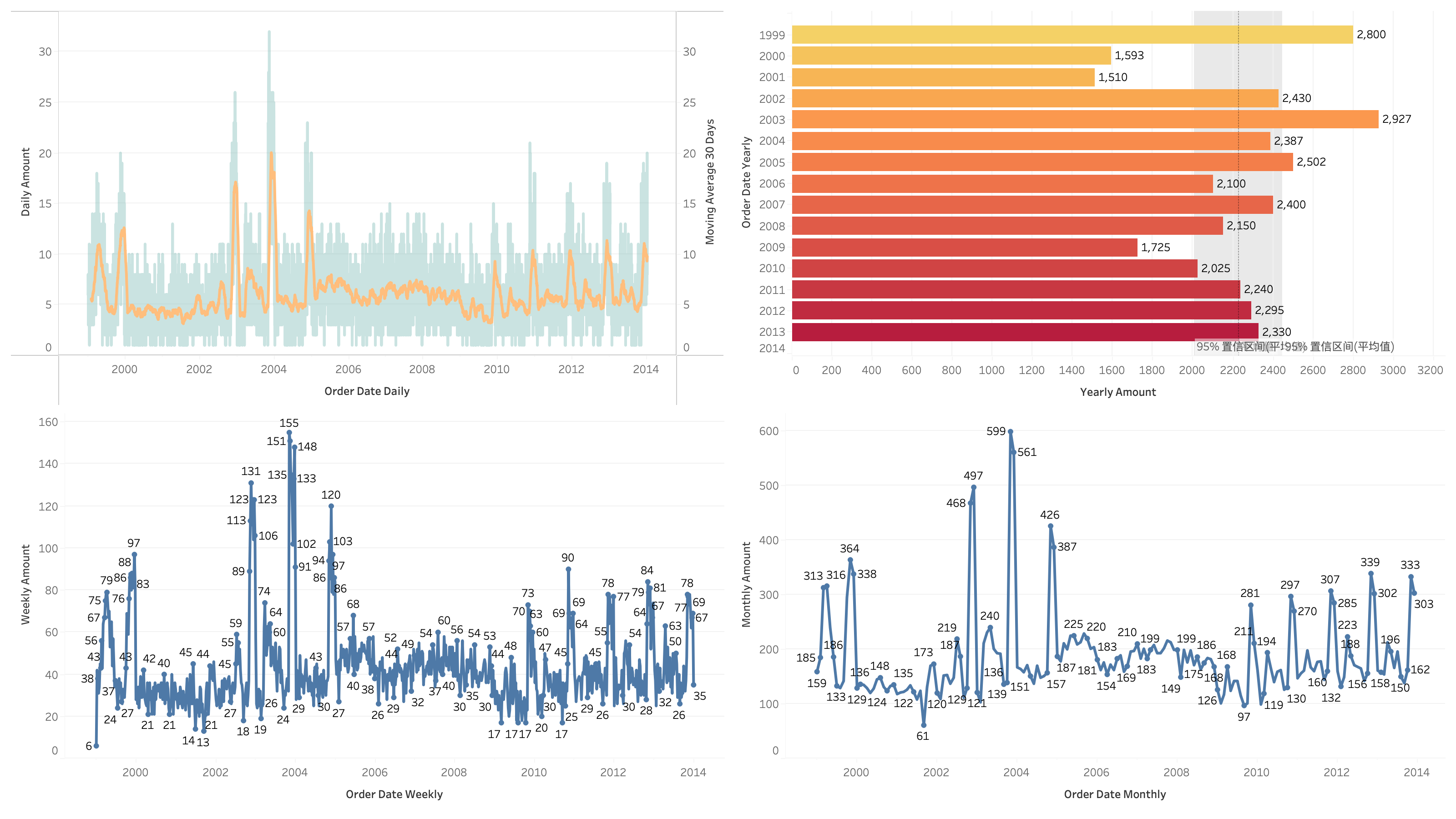
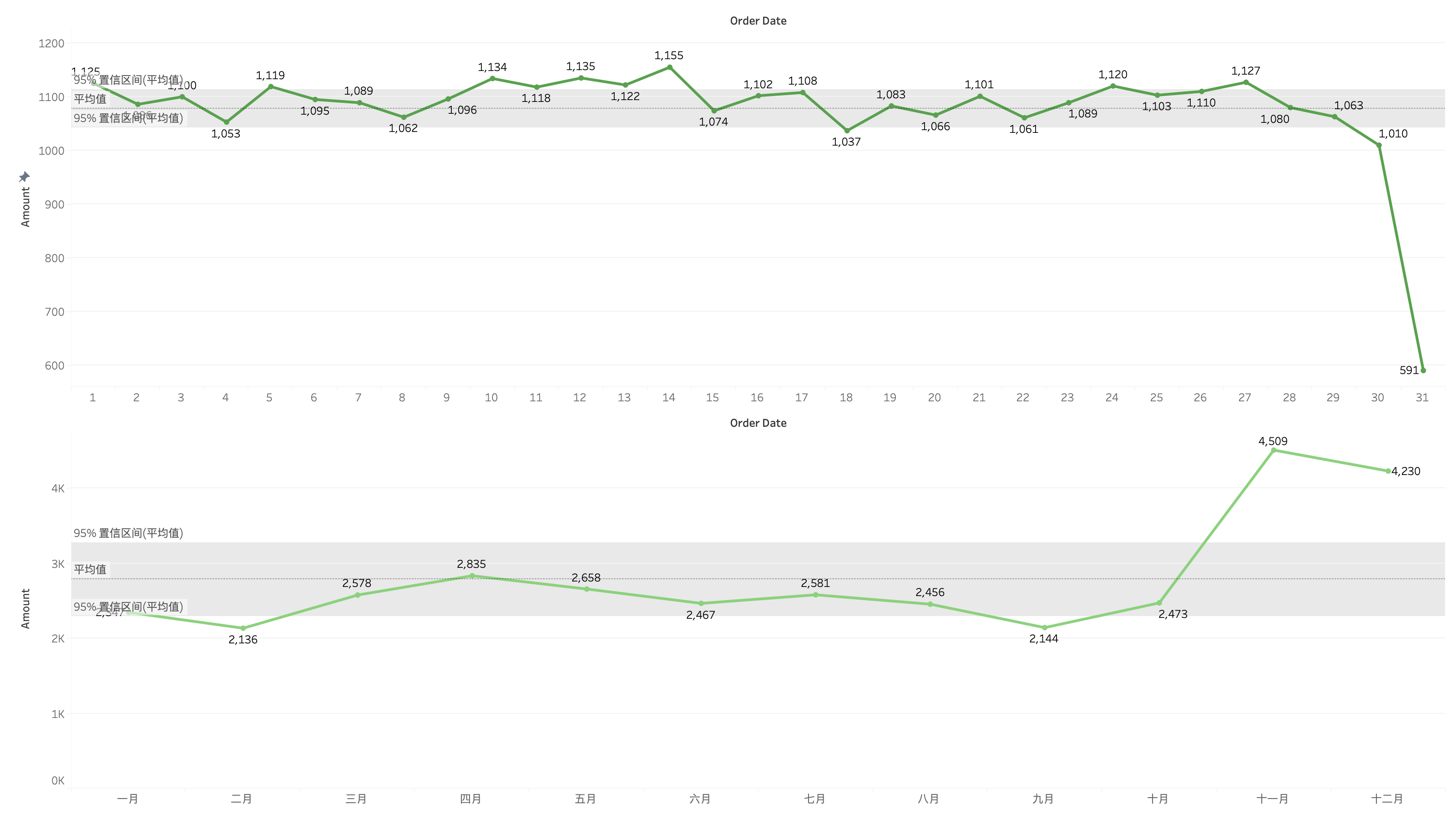
Fig 2-2 shows that, in the end of a month, the sale condition goes downward rapidly, and in the end of a year, the order amounts goes upward rapidly. The weekly sales amouns are about 50 and monthly sales amounts are about 200 to 300.

SELECT S.OrderDate AS OrderDate, S.Year AS [Year], S.Month AS [Month], S.Day AS [Day], sum(S.Amount) AS Amount, sum(S.Profit) AS TotalSell
FROM S2 AS S
GROUP BY S.OrderDate, S.Year, S.Month, S.Day;

2.2.2 Sales Amount: ModelType and Color

The company produces bicycles in 6 types of models and 13 types of colors. Using SQL and Tableau, we can see that the popular trend of each model type and color and their amounts ratio in the whole company.

Among the color, Morning Sun, Hazard Flame, Grey Granite, Fire and Smoke, Copper Haze, Mountain Green, Sea Green Fade, Sky Fire, Arctic White and Wine Country are the main bicycle’s color in the company. Their amounts account about 8% of the total amounts. Some color like Black Hole and Neon Blue are not so popular, whose amounts are about 4% of the total amounts. Each type of color are proportional according to the timeline, which means customers do not prefer specific colors in specific seasons.

Among the model type, Race, Mountain full and Road are the most welcomed model types. Tour and Hybrid bicycles are not main model type in the company. During 2001 to 2012, there is zero Hybrid bicycles produced. However, the company produced Hybrid bicycles again.

SELECT B.Year AS [Year], B.Month AS [Month], B.Color AS Color, sum(B.Amount) AS Amount, sum(B.TotalSell) AS TotalSell, round(TotalSell / Amount, 2) AS AveragePrice
FROM S2 AS B
GROUP BY B.Year, B.Month, B.Color;

SELECT B.Year AS [Year], B.Month AS [Month], B.ModelType, sum(B.Amount) AS Amount, sum(B.TotalSell) AS TotalSell, round(TotalSell / Amount, 2) AS AvgPrice
FROM S2 AS B
GROUP BY B.Year, B.Month, B.ModelType;

2.2.3 Sales Quantity: Volume and Profit

The business volume and the profit are both increasing yearly. The profit are from $1,747,584 in 1999 to $4,217,397 in 2012. The lowest profit rate is 1.92% in 2005. In recent 4 years the profit rate are greater than 20%, which means the company has a great operation condition.

Using simple linear regression and 95% confidence interval, we expect that in 2014, the business volume is about 16 million dollars, the profit is about 3 million dollars and the profit rate are 23.68%.

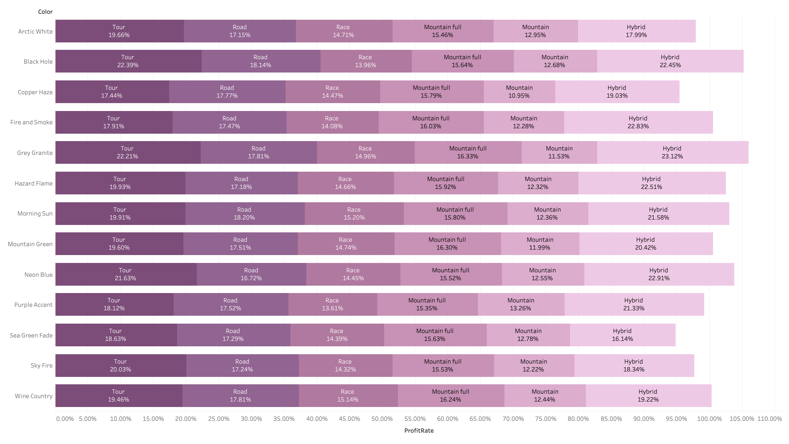
2.2.5 Sale Profit: ModelType and Color

Using SQL and Tableau, the relationship between profit rate and color or model type is figured.

Types of color have no influence to profit rate.

Different types of bicycle model have obviously difference of profit rate. Hybrid and Tour bicycles have the higher profit rate than others. The Mountain bicycle has the lowest profit rate.

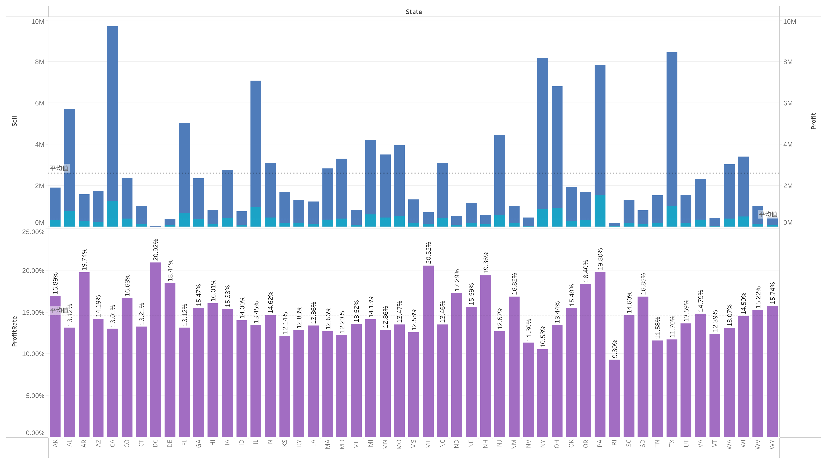
2.2.6 Sale Profit: State

Half of the states have a profit rate above 15%. Some states like AL, CA, IL and TX have a high sale volume. But their profit rate are lower than normal condition of all states. It reveals a phenomenon that when the business in a state becomes huge, the profit rate of this state will decrease. State PA is the unique one which has high business volume and profit rate. The company should make deeply analysis of this state and find out reason why this state is successful to balcance both.

2.3 Conclusion

2.3.1 Sales trend

Commonly, in the end of the year especially the November, the sale amounts of the bicycles achieve the peak. The yearly sales amounts are fluctuating around 2240. The profit are from $1,747,584 in 1999 to $4,217,397 in 2012. In recent 4 years the profit rate are greater than 20%.

The Mountain bicycles are the most welcomed model type and customer has no preference in color of bicycles.

2.3.2 Forecasting

We hope the company will sell at least 2240 bicycles in next year. The sale volume will be 16 million dollars, the profit will be 3 million dollars and the profit rate will be 23.68%.

The company will soonly sell more Hybrid model type bicycles in recent years. With the increasing sale amounts of this type of bicycle, we hope it can be the reason of the company’s profit rate growth.

The company will learn the experience of State PA so that help other states which has a huge business volume increase their profit rate.

3. Ad Hoc Problem Solving

3.1 Retrieve the Data

3.1.1 Search the possible bicycle according to clues

Clues below:

OrderDate	ModelType	State	Color
1998 to now	Rolling Thunder road bike	California	White

SELECT B.OrderDate AS OrderDate, B.SerialNumber AS SerialNumber, B.ModelType AS ModelType, B.FrameSize AS FrameSize, B.TopTube AS TopTube, P.ColorName AS ColorName, P.ColorStyle AS ColorStyle, R.StoreName AS StoreName, R.Address AS StoreAddress, C.State AS StoreState, C.City AS StoreCity, B.CustomName AS CustomName, Cu.Address AS CustomerAddress, Cu.Phone AS CustomerPhone
FROM Bicycle AS B, RetailStore AS R, City AS C, Paint AS P, Customer AS Cu
WHERE (B.ModelType = "Road") and
(B.OrderDate > #1998-01-01#) and
(R.StoreID = B.StoreID) and
(R.CityID = C.CityID) and
(C.State = "CA") and
(P.PaintID = B.PaintID) and
(P.ColorName in ("Arctic White", "Sea Green Fade")) and
(Cu.CustomerID = B.CustomerID)
ORDER BY B.OrderDate;

3.2 Analyze the Data

3.2.1 Divide large group into smaller one (Group By)

In the data retrieving step, bicycles which meet the condition are found. However, there are still a lot of bicycles that match the condition. Therefore, we need to consider other information that do help search the wanted bicycle and its owner.

Among the selected bicycles, all of them are road bicycles. There are two types of color style of them, Sea Green Fade and Arctic White. Policemen can distinguish the style by seeing whether the the bicycle’ s color is white mixed with another color or just white. If it only has one white color, it belongs to the Sea Green Fade color. It not, it belongs to the Arctic White.

After distinguish the bicycle’s color, the group becomes much smaller. To continue divide the group, we need policemen provide further information about which city the bicycle was found and what size the bicycle’s frame and the top tube was.

Fig 3-2 shows the amounts of each smallest group after all information are filled. Most of the option have only one candidate, which means the wanted bicycle can be easily found by further information.

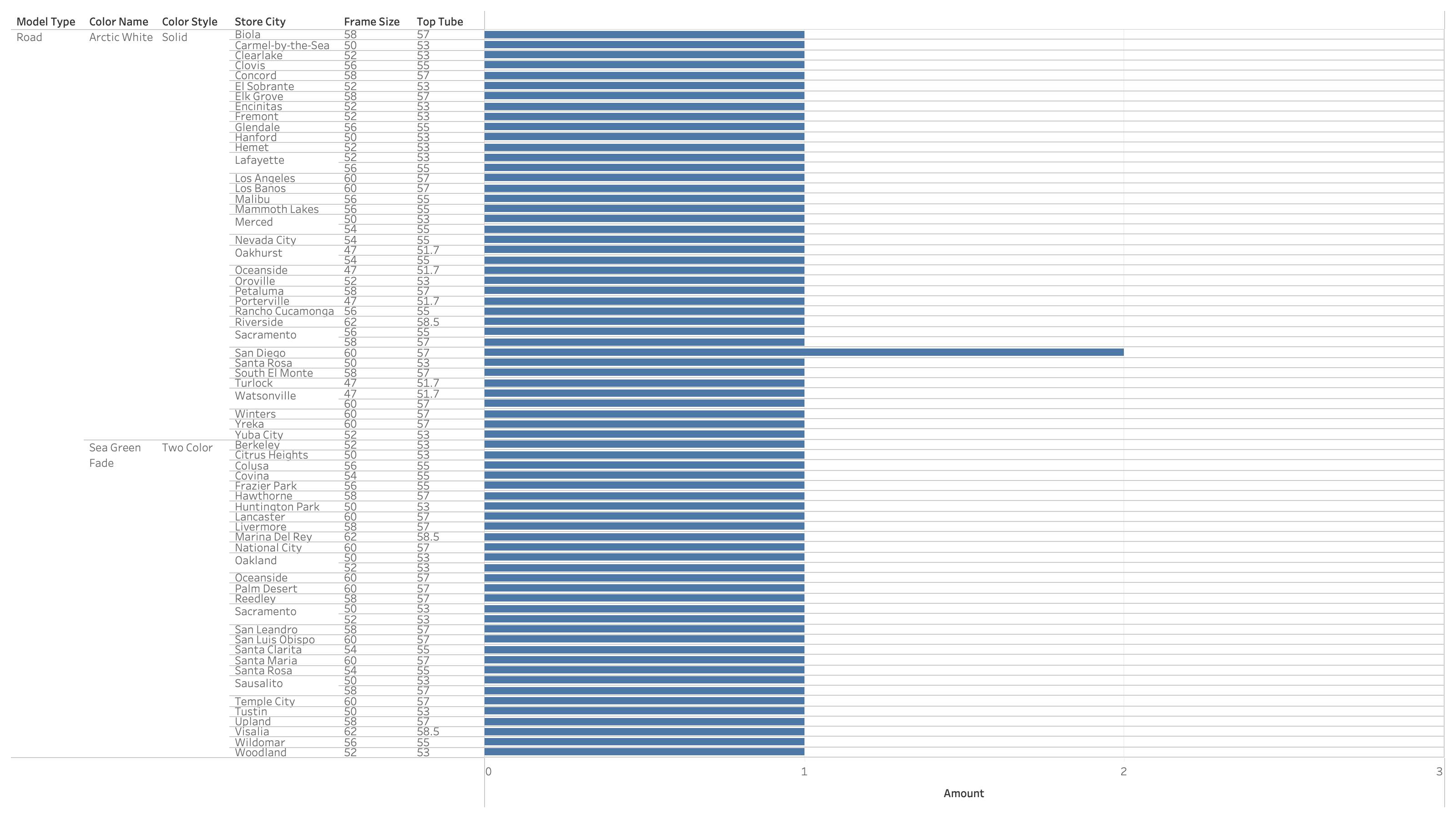
SELECT B.ModelType AS ModelType, B.FrameSize AS FrameSize, B.TopTube AS TopTube, B.ColorName AS ColorName, B.ColorStyle AS ColorStyle, B.StoreCity AS StoreCity, count(*) AS Amount
FROM S3 AS B
GROUP BY B.ModelType, B.FrameSize, B.TopTube, B.ColorName, B.ColorStyle, B.StoreCity
ORDER BY count(*) DESC;

3.3 Conclusion

3.3.1 Find the bicycle

We hope policemen provide further information about frame size, top tube size, color style and city name, and we use SQL to find the corresponded customer.

For example, policemen provides information below.

FrameSize	TopTube	ColorName	City
52	53	Arctic White	Hemet

With the help of SQL (code below), result is quickly found.

CustomName	CustomerAddress	CustomerPhone
Willard Shaffar	3019 Cline Avenue	(314) 602-4259

SELECT B.CustomName AS CustomName, Cu.Address AS CustomerAddress, Cu.Phone AS CustomerPhone
FROM Bicycle AS B, RetailStore AS R, City AS C, Paint AS P, Customer AS Cu
WHERE (B.ModelType = "Road") and (B.OrderDate > #1998-01-01#) and (R.StoreID = B.StoreID) and (R.CityID = C.CityID) and (C.State = "CA") and (P.PaintID = B.PaintID) and (P.ColorName = 'Arctic White') and (Cu.CustomerID = B.CustomerID) and
(B.TopTube = 53) and (B.FrameSize = 52) and (C.City = 'Hemet')
ORDER BY B.OrderDate;

4. Cost, Delivery, and Continuous Improvement

4.1 Retrieve the Data

4.1.1 Days

SELECT B.SerialNumber AS SerialNumber, B.ModelType AS ModelType, B.OrderDate AS OrderDate, B.StartDate AS StartDate, B.ShipDate AS ShipDate, B.SaleState AS State, C.City AS City
FROM Bicycle AS B, RetailStore AS R, City AS C
WHERE (B.StoreID = R.StoreID) and (R.CityID = C.CityID);

SELECT B.SerialNumber AS SerialNumber, B.OrderDate AS OrderDate, (B.StartDate - B.OrderDate) AS PrepareDays, (B.ShipDate - B.StartDate) AS ProcessDays, (B.ShipDate - B.OrderDate) AS TotalDays, B.State AS State, B.City AS City
FROM S4 AS B;

4.2 Analyze the Data

4.2.1 Prepared days shortening

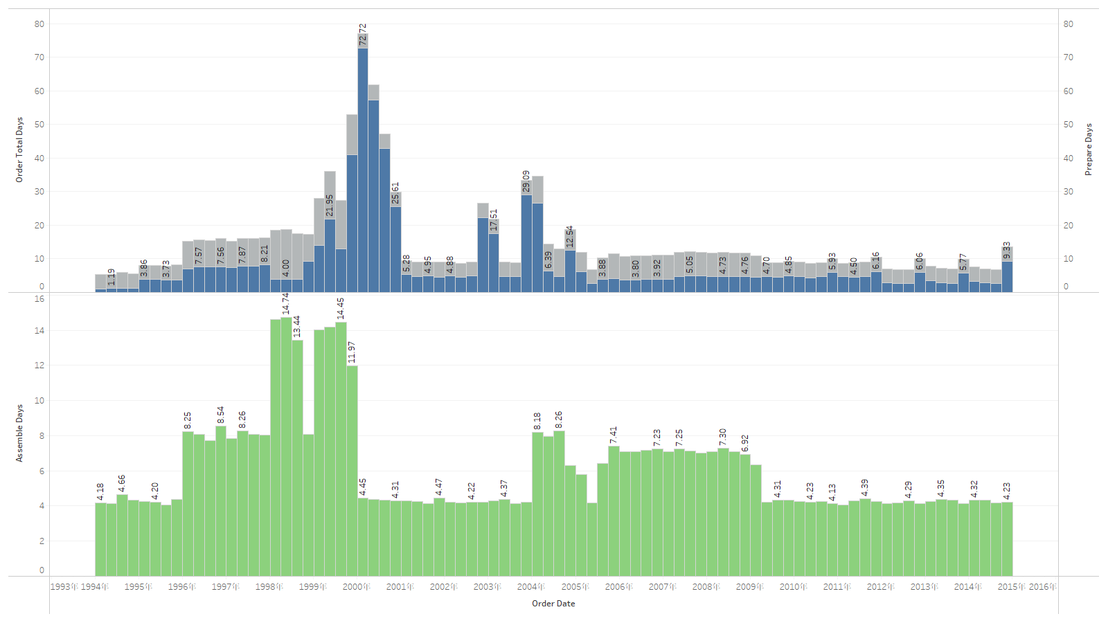
According to the data of OrderDate, StartDate and ShipDate, we can compute the component preparing days, assembling days and total days. The less total days, customer receives their bicycles sooner. Therefore, it is important to derease both the component preparing days and assmebling days.

Using SQL, we can easily find the average component preparing days and assmebling day for each season. In Fig 4-1, it shows that the data between 1999 to 2001 have a irregular value, which means these data are obviously the dirty data. Therefore, we only use the data in other time period. The average assembling days of each seasons are surrounding 4 or 5 days, which is already stable and performs well. But the data of component preparing days have a great space of shortening the time. In Winter season of each year, the component preparing days are greatly increasing. It shows a bad performance of the company’s inventory ability in Winter. Therefore, the company need to redesign the inventory plan and store more components in Winter.

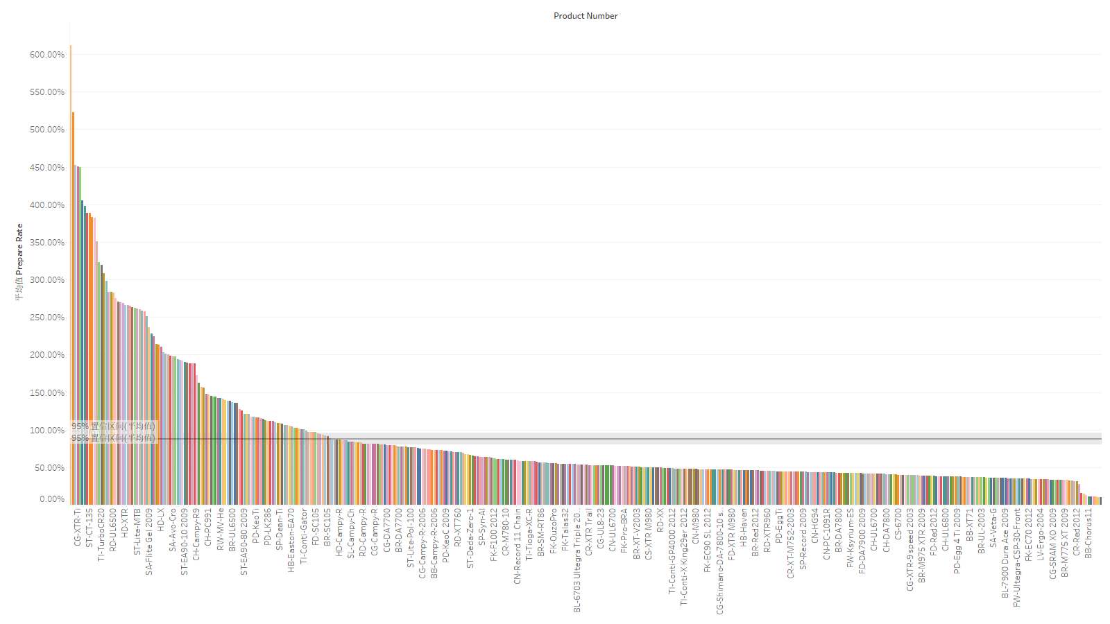
Then, we consider how to adjust the amounts of components in the inventory. First, we estimate the amounts of components used in next one year. The data of component usage in the last year is a good estimator. Therefore, we can use SQL to retrieve the data of component uage in the last year. Second, we use SQL to retrieve the data of the quantity of components in the inventory. Third, we compare these two values and define a Prepared Rate = QuantityOnHand / Usage of Component. This ratio reveal the condition how a component is prepared in enough amounts. Finally, we set 79.97% , which is the upward bound of 95% confidence interval as the standard prepared rate.

The company can build a Enterprise Resource Planning Systems to assign component purchasing orders to each inventory. After using this system, the amounts of most of the components are always enough. And it will greatly shorten the component preparing days, and thus shorten the delivery days to improve customer’s experiences.

SELECT O.ComponentID, C.ProductNumber, O.QuantityUsed, C.QuantityOnHand, FormatPercent(C.QuantityOnHand / O.QuantityUsed) AS PrepareRate
FROM (select C.ComponentID as ComponentID, count(*) as QuantityUsed
from (select * from Bicycle B where B.OrderDate > #2014-01-01#) as B, BikeParts as BP, Component C
where B.SerialNumber = BP.SerialNumber and
BP.ComponentID = C.ComponentID
group by C.ComponentID)  AS O, Component AS C
WHERE O.ComponentID = C.ComponentID or
(C.ComponentID not in (select C.ComponentID as ComponentID from (select * from Bicycle B where B.OrderDate > #2014-01-01#) as B, BikeParts as BP, Component C where B.SerialNumber = BP.SerialNumber and
BP.ComponentID = C.ComponentID
group by C.ComponentID) and
C.QuantityOnHand > 100);

4.2.2 Cost decreasing: RetailStore

In 2.2.6, we already have the conclusion that areas which have high business volume have low pofit rate. In order to decrease the cost, we can cut down some retail stores in such areas.

Using SQL, we select city with CityID 197, 214, 639, 784, 3011, 3988, 4515, 4739, 5065, ... In this city, we cut one nineteenth amounts of retail store which is totally 19 retail stores. Assume that cutting down each retail store can save 40 thousand dollars for shipping cost and daily operation each year, it will save almost 0.76 million dollars.

SELECT RetailStore.CityID, Count(*) AS Amounts
FROM RetailStore
GROUP BY RetailStore.CityID
HAVING (((Count(*))>19));

4.2.3 Cost decreasing: Component discount

While purchasing the component, it is usually having a discount. In 2014, the yearly component cost is $7,224,258 and the discount rate is 2.51%. If in next year, the company can ask partner for better discount and let the discount rate increase to 3.00%, the company can save approximately 36 thousands dollars.

SELECT sum(TotalList) AS Total, FormatPercent(sum(Discount) / sum(TotalList)) AS DiscountRate, sum(TotalList) * 0.005 AS Expected
FROM PurchaseOrder
WHERE OrderDate > #2014-01-01#;

4.3 Conclusion

4.3.1 Data collecting

To avoid the situation like dirty data of orderdate from 1999 to 2001, the company will build a new Logistics and Distribution system to record each order data of saled bicycles. Each manufacturer will join in the new Parter Relationship Management and use the same standard to record assembling data.

In the BikeParts of the Database, the SubstitudeID column exists but with all zero values. If this data can provide the meaningful information, we can continue decrease the cost of the company by using substituted components. Therefore, the clerks should fill the SubstituteID data in the database.

4.3.2 Delivery days shortening

Through the ERP system, inventory make each prepared rate of components around 79.97%. After this new system is equipped, we expect the component preparing days decreased a lot.

4.3.3 Cost decreasing

Assuming the total cost of the company is same as in 2014 and is 9 million dollars. After cutting down the amounts of retail store and purchasing the components in a better price, the company can save approximately 8.84% of cost.

select FormatPercent((36000+19 * 40000) / 9000000)
from S4;

5. Appendix

The original SQL is in the Access file. The SQL is also transferred as Excel file.

Each Figure and its Tableau file is in the Zip file.